Understanding Variable Life Insurance: Part 1

The National Association of Insurance Commissioners (NAIC) spent almost five years developing the Model Illustration Regulations currently in use - in one form or another - in most states. The regulations were developed to help the consumer have a better understanding of how Life insurance policies worked, as well as to better differentiate between guaranteed and non-guaranteed elements of a Life insurance policy.

These regulations, which generally cover policies sold after January 1, 1997 (or a later date as enacted by individual states), include all forms of individually sold Life insurance exceptthose policies which fall under the jurisdiction of the National Association of Securities Dealers (NASD). The NASD regulates illustrations for "registered" Life insurance policies - popularly known as variable policies. The NAIC has intended to reconcile differences between their Model Illustration Regulations and the regulations of the NASD, but to date the level of cooperation necessary to develop joint regulations hasn’t occurred.

Variable Life insurance illustrations enjoy a unique "franchise" from the NASD: only this type of registered product may be specifically illustrated for future value projections. Mutual funds, individual securities, and even variable annuity products are not covered by the exemption from rules prohibiting the projection of future values. Variable Life insurance policies may be illustrated at a rate not to exceed a gross average rate of 12%, and a 0% rate and a mid-point rate must also be shown. Of course, a variable Life insurance policy discussion can’t take place without first providing a prospectus to the potential buyer of such an investment. These illustration regulations allow the buyer to better understand "how the policy works" while at the same time protecting against unreasonable projection of values.

The major problem with the regulations covering Variable Life insurance policy illustrations is that the allowable investment return rate used - up to but not exceeding 12% gross - is defined as a constant average rate. That is, whether it’s a 4% gross or 12% gross, the same rate must be applied uniformly for all years.

To better anticipate actual Variable Life insurance (as differentiated from policy projections), it’s important to understand long-term market performance. Can you answer these questions?

• From 1926 to 1998, what was the total annual compounded return of Large Capitalization Stocks in the U.S.?
• How about for the period 1960 to 1998?
• The period 1970 to 1998?

The correct answers are around 11% for 1926-1998, around 12% for 1960-1998, and around 13.5% for 1970-1998.

SO WHAT?

Certainly the long-term historical experience (warning: historical experience is not a predictor of future performance) of the stock market would suggest that 12% rates of return aren’t just a short-term 90s-style phenomenon. ("So, wouldn’t you agree, Ms. Prospect, that if I allow for the average offset for ‘gross’ to ‘net’ returns in Variable Life insurance policies of about 200 basis points, a net assumed policy crediting rate of 10% is not unreasonable given historic, long-term performance?")

Here’s where the trouble starts. If I take just $1,000 and achieve a long-term average rate of return of 11.2% over 73 years, I should have a cool $2.3 million for my trouble. Where’s that time machine when I need it? But do the same "laws" of compound interest apply to the mechanics of Variable Life insurance?

The answer is an emphatic no! Both because of the monthly "disinvestments" that occur as Cost-of-Insurance (COI) charges are liquidated out of the sub-accounts and because of the mysteries of the Net Amount at Risk - unique to Life insurance - our expectations won’t be realized merely for a given assumed rate of return.

A BRIEF DIVERSION INTO NET AMOUNT AT RISK

The magic of Whole Life (or any "permanent"/cash value-type of Life policy) is that as the cost of the risk element goes up (due to the increasing probability - as we get older - that death might occur this year), the risk element of the policy is decreasing due to an increasing cash value. In variable plans of Universal Life insurance illustrated at 12% gross, the cash value needs to be roughly 50% of the death benefit at life expectancy if the plan is to "endow at age 100." (Age 100 is an actuary’s view of "lifetime sufficiency.") But variable universal Life-type policy cash values are subject to fluctuation without ceiling (or floor). What if the cash value should drop 20% at Life expectancy - at age 89 in this example?

For a 57-year old female (non-smoker)

End of Year Cash Value % Chg Net Amt @ Risk % Chg Death Benefit

32 530,000 470,000 $1 million

33 424,000 -20% 576,000 +23% $1 million

The COI charge at the end of year 32 is $39,500 ($83.50 per $1,000). The effect of a 20% decrease in cash value is to increase the Net Amount at Risk by a higher factor. The following year’s COI will apply to a substantially higher Net Amount at Risk and the resulting stress on the underlying Life insurance policy is such that it’ll lapse in a few years unless a "premium" comparable to the loss of cash value is promptly injected into the policy.

BRINGING IT ALL TOGETHER

Appropriate disclosure and examples that cash values can and will fluctuate in a variable universal Life policy is essential to determine the prospective policy owner’s suitability for this type of Life insurance. The possible negative effect of cash value fluctuation - especially on "thinly funded" policies - is just as important.

This graph of paid cumulative premium, cash value, and death benefit depicts the earlier example of a 57-F-NS with a $1 million variable universal Life policy. Annual premiums and the resulting cash values are calculated using a constant average 12% gross investment return. Although depicted graphically rather than numerically, the illustrated result with a minimum annual premium is consistent with current NASD requirements regarding policy illustrations.



 

The next graphic portrayal illustrates the same policy and premium flow, but with the constant average 12% gross replaced with actual "large cap" equity market monthly returns - from 1956 to 1998. These monthly returns are applied in the sequence in which they occurred to the 43-year period from policy issue to policy maturity. By the way, the index itself would result in a compounded average return of 11.9% for the 43 years in this example.



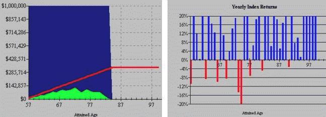
The greatest concern over the hypothetical result is that it’s inconsistent with current regulations regarding what may be shown to a client. So Registered Representatives are barred from calculating or demonstrating this possibility to their clients. At the same time, however, it’s critical to understand that the negative effect suggested in this graphic scenario does not suggest that variable Life products are unduly risky or "bad."

In the next article, we’ll continue to explore the intricacies of variable Life insurance from the standpoint of regulation and reality - and to find client-focused solutions for these otherwise unfavorable possible results.